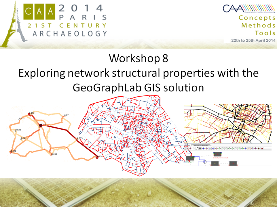
GeoGraphLab : main presentation
Exploration scenario : the 1300 Paris network
A very first measure : betweenness centrality
Filter a source node to set the OD-space
A second measure : the average distance
A third measure : the degree centrality
Combined measures: a way to create new dedicated measures
Export results to shapefile (or others file format)
A case-study : supply and diffusion of goods through the network
Contacts : eric.mermet@ehess.fr, sandrine.robert@ehess.fr
Link to the main presentation : pdf
Please : use the google document share here if you want to correct english mistakes...
This workshop proposition is linked with the transportation network analysis session. GIS solutions are growing with the emergence of open source software. These tools offers analysis methods in various domains involving geolocalised data. On a network, data are nodes, edges. These data structures can be studied simply, some might say too simply, by graph theory[Berge, 1973] developed in the late 1950’s.
It is interesting to notice that first studies using graph theory and very beginning of GIS focus on an historical view of the medieval river trade network of Russia [Pitts, 1965] [Pitts, 1978]. In such a study, it is highlighted, with various network measures like (accessibility, centrality, proximity) that the special position of the city of Moscow in the river system led to affirm its economic dominance and became capital.
Other methods of analysis of networks add a relational dimension to the simple graph theory [FreeMan, 1979] [Sheffi, 1984] [Bolobas, 1998] . If this dimension adds a combinatorial complexity, the most interest is that it becomes possible to understand phenomena underpinned by the only network effect [Gleyze, 2005] without the need to integrate thematic data. While at present it is becoming easier to integrate open and free data in GIS tools (travel surveys, GPS tracking, etc.), obtaining reliable historical data often falls many years of hard work and research documentation of confidence.
In this workshop, we propose to introduce a tool for analyzing relational phenomena on networks. GeoGraphLab [Mermet, 2011] is a complete open source GIS solution that allows to analyse and to map networks without thematic data based only on its structural properties. Indeed, a network due to its intrinsic properties reacts in its own and unique way to different stimuli. These reactions are dictated by the arrangement of the network components and how these components are activated by relationship: that's what we call the potential relational network.
This approach is based on the geometric aspect of components nodes (positions) and edges (geometries), topological aspect (edges connect nodes), metrics aspect (length, time, costs, etc..) and finally relational aspect (all the relations on the network have to be considered). Then relations are reflected by paths (shortest paths, random paths, etc..) for which it is possible to measure properties to obtain indicators on the network (like betweenness or proximity centrality, average distance, distal or proximal radius, etc..). These indicators, once mapped, offer a particular view of the network status in the study.
Different pretreatments are integrated to correct topology, induce a metric, to check the connection. It is also possible to filter relations, to take an interest in specific phenomena involving a set of relations of interest. Finally, an integrated tool for crossing created maps will be presented as a complete graphical language in order to speed up studies and network analysis.
This tool called GeoGraphLab (GGL) with be used on a study of the Paris network in early XIVè century. We will show a large panel of the tool possibilities.
The first step is to install Java :
https://www.java.com/fr/download/
Java is already configured on the workshop computers. So pass, this step if you plan to work with these computers.
Download the latest version of GeoGraphLab here :
http://geographlab.free.fr/caa2014/GeoGraphLab-0.4-SNAPSHOT.jar
Download the data here:
http://geographlab.free.fr/caa2014/data_W08_CAA2014.zip
This file is a jar (Java archive), so it can be run on any platform (Windows, Mac, Linux).
To start the program, you normally have to simply double-click on it. After few seconds, GeoGraphLab will start.
BUT, this running mode do not allow to define allocated memory for GGL.
GeoGraphLab needs a lot of memory if you want to work with large networks, more you make and store calculations, more you need memory.
The ideal memory configuration is something like Intel I7 with 16GB RAM.
But for these 4GB limited computers, we will allocate 2GB for GeoGraphLab.
In Windows run under a terminal (type cmd on the “execute” menu).
And enter this expression :
java -jar -Xmx2G GeoGraphLab-0.4-SNAPSHOT.jar
GeoGraphLab is a tool built on the top of the conceptual model presented earlier. It is a multiplatform tool as it is written in Java and use common LGPL libraries like JGrapht[1] that
provides us mathematical graph-theory objects and algorithms, GeoTools[2] and JTS[3] for spatial analysis.
Different features for Human-Machine Interface has been implemented in this tool like: loading a network files (Shapefiles), allowing graphical interactions like drag and zoom, adding or removing components (nodes, edges, aggregate areas), modifying attributes of components (names, colors, weights), putting a background map or image, changing legends for maps created, docking windows for users customization of his own workspace.
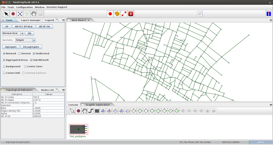
When you run GeoGraphLab, you should get the following window, which is the main window.
1 - Draw a network, select components, drag and zoom
GGL is as a tool for analyzing networks, so you can draw your own network node by node, and connect nodes with edges. You can find all you need in the mail toolbar :
Draw nodes, aggregate selected nodes into one node, draw edges and delete selected objects.
Try to draw a test network.
If you want to select node, first select the associated tool. You can select multiple nodes by keeping shift key pressed.
Once you have selected one node, you can move it with the tool “move node”, or if multiple selected nodes, it will move the last selected.
The two following tools allow special selections :
- select neighbours of the selected nodes.
- select the minimum spanning tree of a selected node.
Next buttons allow to drag with right click and to center the network view.
You can also drag by pushing the central button regardless of the selected tool.
Zooms and de-zooms can be obtain with the central mouse wheel.
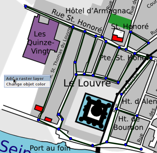
2 - Use a raster layer as a model
You can display a raster layer as a mask to create you own network.
Just right click on a blank area and choose a file, for example you can train with the CarteParis1300-1330.png file.
3 - Shortest path
Now that your network has been entered, you can select two nodes with the shift key pressed.
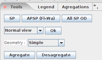
In the tool panel, the button SP (shortest path) can be used to compute the shortest path between the two selected node.
4 - Aggregate/Disaggregate
It is possible to combine visually nodes in an aggregate node.
First, select several neighbours nodes and click the Aggregate button.
If you want to disaggregate nodes, juste select one the aggregated node and click Disaggregate.
5 - Loading Shapefile
GeoGraphLab is shapefile friendly. It is possible to load LineString geometries as network.
While loading shapefile, GGL build the graph structure, that’s why it’s a slower than loading data under GIS. It’s only when this structure is built that we can compute shortest paths and measures.
Try to load any shapefile you want via the menu File/Open Shapefile …
For example, choose the test_network.shp file in the testShape directory.
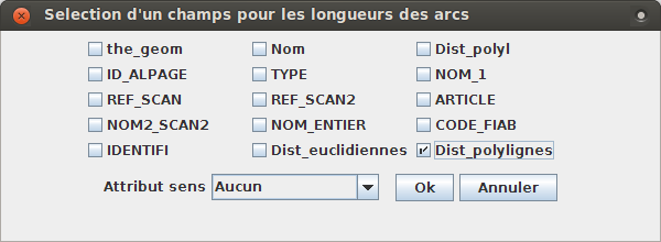
A window ask you to select what attributes you want to load. You can select several attributes providing that it is numerical values, not text values.
For this example, choose dist_polylines. It will ask to GGL to autoweight edges with the length of lines of the network. The calculus is 3D based on x,y,z coordinates.
6- Applying pre-treatments
The first thing to do is to be sure that the topology is sure. If the topology is not correct, the network will be separated with too many connected components. To be sure that all points will be linked with all others, it is needed to have exactly one connected component.
GeoGraphLab can assist users in filtering network to be fully compatible with algorithms.
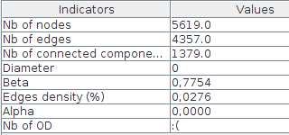
These information can be checked in the topological indicators :
In this example, the loaded network has 1379 connected components. It is far too much !
A path must exists between any node on the network. We need to fix that !
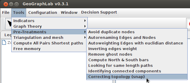
This filtering step is separated into two actions :
- Correcting topology by snapping geometry nodes :
- Identifying connected components, the tool will automatically select the biggest connected set.
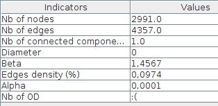
After these two pre-treatments, the topological indicators will show :
Once pre-treaments has been computed, graph has exactly one connected set of components, you can try shortest path between two nodes in order to test the network.
“Alpage” Project (diachronic analysis of the Paris urban area: a geomatic approach) : http://alpage.huma-num.fr/fr/
A lot of historical data about Paris have been georeferenced and vectorised : click on the map : http://dmap.tge-adonis.fr/alpage_public/flash/
http://alpage.huma-num.fr/fr/ressources : Cartes : Cartes générales :
http://alpage.huma-num.fr/documents/ressources/cartes/CarteParis1300-1330.pdf
Noizet, Hélène. « Les relations entre la ville et le fleuve à Paris de l’Antiquité gallo-romaine au Moyen Âge central ». Les Nouvelles de l’archéologie 125 (2011): 32‑40.
http://halshs.archives-ouvertes.fr/docs/00/66/85/48/PDF/Noizet_NouvArcheo.pdf
See figure 4 : Principaux tracés viaires en rive droite
The data layer for the Paris street 1300 is on : http://dmap.tge-adonis.fr/alpage_public/flash/
Export SIG : Voies 1300 : L’intégralité : ESRI Shape
Go to the data folder CAA2014/Couches1300 of the workshop and load the file called : voirie1300.shp.
Please apply the two pre-treatments seen above : topology snapping and connected component identifying.
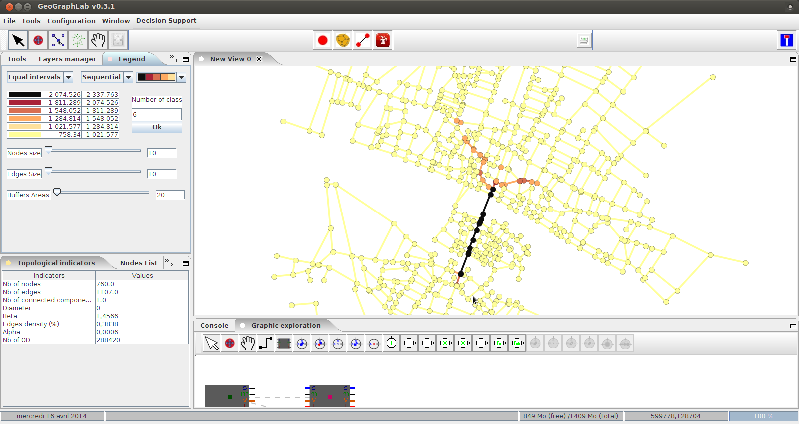
GeoGraphLab will normally display something like that in the topological indicators :
760 nodes
1107 edges
1 connected component
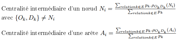
Betweenness centrality quantifies the number of times a node or an edge acts as a bridge along the shortest path between two other nodes.
This measure is defined by :
More a component of the network will be crossed by shortest paths, the more it will be a necessary component in relationships between nodes. These components of the network (nodes or edges) will be central or essential.
For more details about network measures, you can refer to :
- Social network analysis, Wasserman & Faust :
http://books.google.fr/books/about/Social_Network_Analysis.html?id=CAm2DpIqRUIC&redir_esc=y
- Or my phd work (Annex A), only in french :
http://recherche.ign.fr/labos/cogit/pdf/THESES/MERMET/theseMermet2011.pdf
To do that, it is needed beforehand to compute all pairs shortest path. It is the classical betweenness centrality.
In GeoGraphLab, you can compute all pair shortest paths (APSP algorithm) with a single button.
You can find it in the Tools panel as APSP (Fl-Wa). Fl-Wa means that the algorithm used is based on the Floyd-Warshall classic algorithm enriched with a multi-processor computing.
The shortest paths will be computed, you can check if it’s ok in the bottom right progress bar of the application. Sometimes, it may happen that the progress bar will not move. Please be patient. After few seconds, you may observe progress bar move.
After approximatively 1 min, around 288000 shortest paths have been computed. Once reach 100%, you can go on.
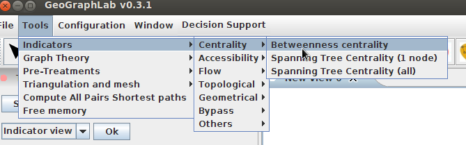
You can now start the betweenness centrality computation. You can find the option in Tools/Indicators/Centrality/Betweenness centrality, as follow :
Since shortest paths has been pre-calculated, betweenness centrality is very quick to finish.
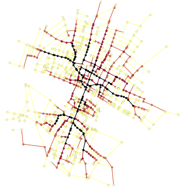
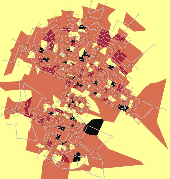
You can observe the resulting map :
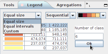
This map is not very clear because of the equal size legend classification. Nevertheless, it appears that the more central components are mainly located around the two north-south bridged.
To observe others phenomena, you can easily change legend in the Legend panel. Now choose an equal size classification and click Ok, as follow :
What do you observe ? Discussion.
This structure of shapes is very characteristic on how the network reacts to all shortest paths and each network reacts differently.
Now that you have obtain betweenness centrality on the full OD-space, it means that all the shortest paths have been computed, you can filter and reduce the OD-space to what you want.
Imagine you want to focus on a particular node, you can obtain a new betweenness centrality one one node very easily with GeoGraphLab. To do that, you have to go to the “Console panel” which is near the graphic exploration panel.
In this panel, it is possible to enter commands. For example, type help to get a list of proposed commands.
If a block-map is selected, you can type espace[4].
You will obtain the size of the OD-space, this size is back and forth OD.
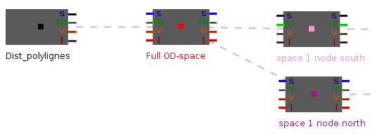
In GGL, you can create or remove block-maps with this button
Now, create two block-maps with the add block button to obtain this schema :
Note that you can rename the created block-maps in layers manager panel by double-clicking and name.
Now select one of the new block and go to the console panel.
Select a node in northern network , its name will be displayed in the console, for example V_xxx.
Now type in the console this line :
> filtre espace n V_xxx
Do the same thing with an other node in the southern network.
If you type espace after selecting one of this new block-map, you will obtain a new size. If it’s ok, it will display 759 ODs.
You can now obtain betweenness centrality on the new filtered relational space just by choosing indicator in the menu.
Betweenness centrality for a north node | Betweenness centrality for a south node |
GGL gives tool to easily combined visual block-maps. Now that you have created two centrality measures with two different relational space, you can cross their OD-space.
In GeoGraphLab, you can work on map-blocks with the dedicated toolbar :
In ordered icons: select or move block, drag the interface, you can connect blocks to others blocks or to operators, create or delete blocks, and finally add blue operators (set theory operator for maps relational space : combine Origin-Destination set) or green operators (mathematical operations on measures). Blue operators allows to connect blue connectors on block-maps and green operators allows to connect green connectors. Others colored operators are not yet available at the moment.
For operations on OD-space, operators are available like union, intersection, difference, etc.
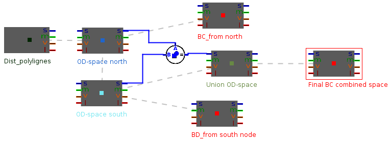
You can try with this exploration schema :
In order to save memory, please delete the last blocks we have created and keep the betweenness centrality on the full OD-space.
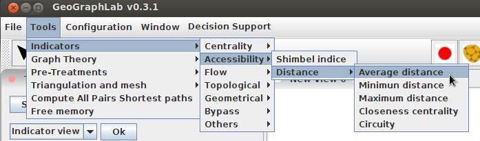
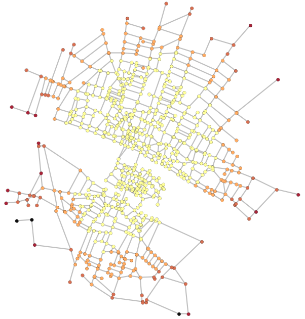
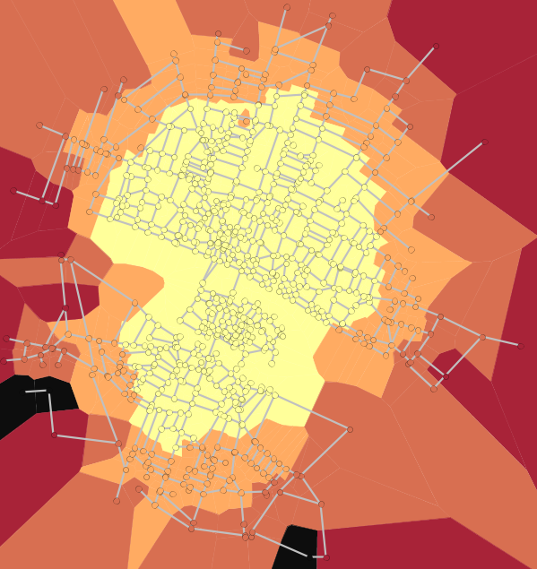
In the same idea, you can now compute the average distance. Average distance is an accessibility measure. For each node, we compute the distance to each other node and then we average distances.
If all is ok, you will normally obtain this map as result :
You can aggregate result on nodes on its Voronoï surface. Voronoï surface represents relatives euclidean spatial dependencies on nodes.
To do that, first you have to activate the voronoi int the tool panel. Then click on “Coloring Surface” to relative to the displayed measure. You obtain the second map presented above.
This map show the concentric formation of the Paris network. More an surface is dark, more its distance to each other node is high, less the node is accessible on the network.
The two measure we have first computed are based on relational properties of the network, basically all the shortest paths in our case.
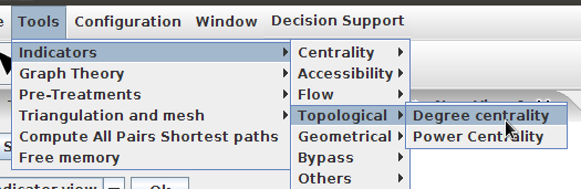
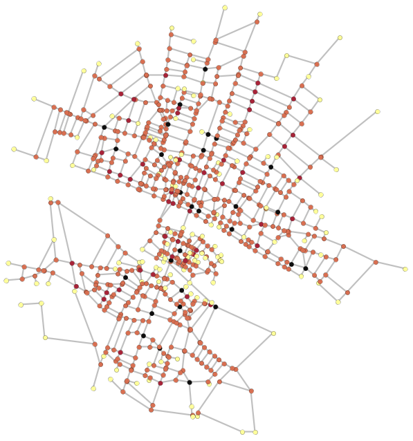
More simple indicators are allowed and can also be computed in GeoGraphLab. For example, a very basic measure is the degree centrality. It computes the number of neighbors for each node. Logically, more a degree have neighbors, more it will be a central node. But this is not so simple in network analysis. The measure is not sufficient to conclude on how networks react to stimulation or can explain phenomenon.
So, to compute the degree centrality, simply follow the menu :
You can obtain this two maps, following activation of Voronoï cells: black nodes for high degree, lighter nodes for low degree (dead-end street or node on a simple street).
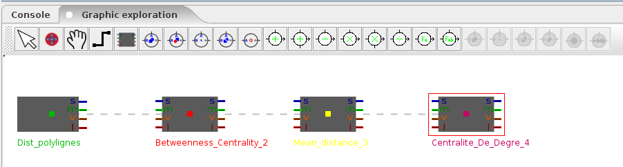
Now, if you look at the graphic exploration panel, you can observe block-maps connected together with light gray dashed lines. Each block have a name (the measure name), and red, green, orange and red connectors.
Dashed lines means that block-maps are derived from a parent block-map.
Others connectors may be used to create new maps with derived properties of other block-maps.
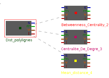
Following the derivation of maps, you can observe different patterns. One may be linear, the other can be as a tree.
Each measure is derived in a linear way.
Each measure is derived from the parent map.
A fast way to obtain a new measure is to reuse ever calculated measures.
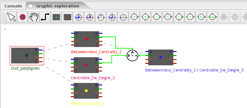
In this example, we want to normalise betweenness centrality with degree centrality.
As we seen before betweenness centrality represents number of paths on each network components. Degree centrality is the number of neighbours for each nodes.
If we divide Betweenness by Degree, we will aggregate information only at a node level and obtain a kind of betweenness centrality / degree, or a kind of average betweenness centrality of edges relatives to its connected nodes.
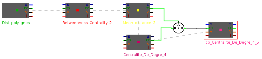
Use the correct operator to compute the desired operation and reorganise your block-maps in order to obtain, something like that :
And observe yout new measure result immediately in the display area.
Computation between two indicators, reorganise map-blocks and connect mean distance and
degree centrality with a mathematical operator block (division).
GeoGraphLab-0.4-SNAPSHOT
Simply use the File/Export menu. You can find Shp or Svg exports.
You just have to select an export file, and choose Ok.
Attention ! Be careful to choose the real geometry on each map you created if you want to conserve the shape of edges.
GGL export two shapefiles, one for edges, one for the nodes. Each attributes will correspond to each block-map you have created.
You can now load these exported results in your favorite GIS software. Here’s an example on QGIS, the combined visualisation of centrality on edges and average distance on nodes.
Qgis view crossed betweenness centrality and average distance | ArcGis view with the same information with an added interpolation on average distance |
Context :
In the second half of the twelfth century . and throughout the thirteenth century during the reigns of Philip Augustus (1180-1223), St. Louis (1226-1270), Philip III (1270-1285) and Philip IV the Fair (1285-1314) throughout the "Beautiful Middle Age" Paris knows a very important development. Quadruple its population.
A wall was built by Philippe-Auguste to protect a growing city, especially on the right side, around the Halles that the king reorganized. Throughout the thirteenth century. They see themselves build new specialized by type of goods and buildings take the grip and appearance they retain until the nineteenth century.
The university, on the left side of the river, colleges welcome students from all over Europe and make Paris the great intellectual center of the medieval West Cf University. The mendicant orders, the Dominicans and Franciscans settled on the left bank and offer new models of preaching, knowledge and poverty.[5]
The short study we want to implement is linked to these two aspects of the city. First we have a supply of goods from West and North behind the wall to Les Halles and the Place de Grève.
And finally markets provide foods and goods to the abbeys on the south by crossing the two bridges.
In order to study this phenomenon, we do not want to compute all paths on the network, but we want to be more specific on what we are looking for. GGL can help to load relationships for which we will interested in.
Quit GGL Start with a new GGL session.
Realise actions in this order :
- Load the Voirie1300.shp network with the dist_polylines features.
- Derive the block-map created with the add map button and obtain cp_Dist_polylines_n.
In Qgis, you can observe the prepared files for this study. Open the MarketsDiffusion_Paris1300.qgs Qgis project.
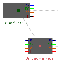
A map of load of goods from around Paris to the two marketplaces (Les halles and Place de grève) in green, and absorption or (markets unload) in red by three main abbey in the left south side of the river Seine.
The idea now is to load on the two created block-map a specific OD-space. First select the loadMarket block and choose File/Add OD Layer. Browse to the provided file points_load_markets.shp and click Ok.
You can observe in the OD list panel that only a limited OD has been loaded.
Repeat the operation for the other block-map with points_unload_markets.shp File.
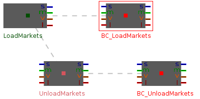
Now you only have to select a block-map and to choose for example a measure of betweenness centrality. Do it for the block-maps and observe the results.
The exploration schema for this study must be something like that :
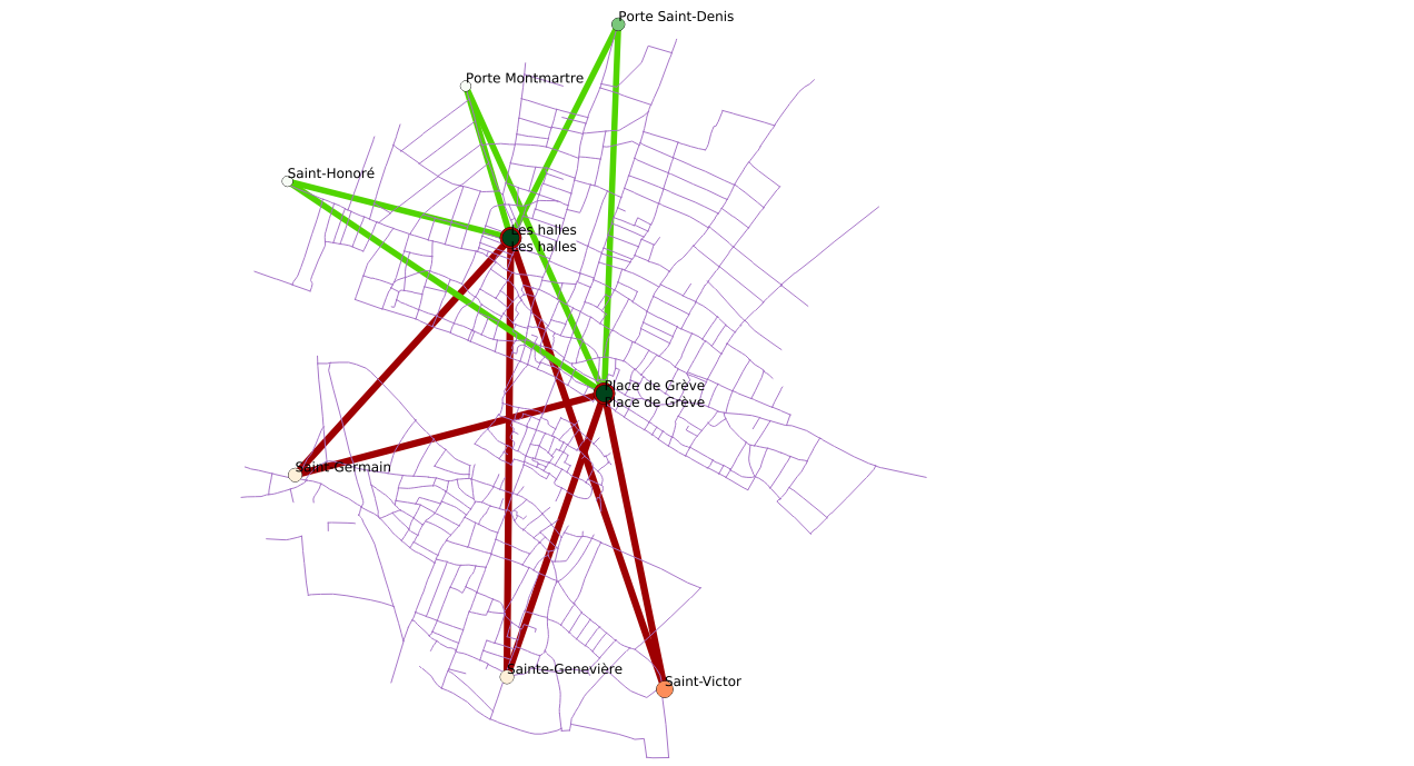
And the results displayed for these measures on the network. This shape of lines are what we call relational signature for the OD-space of interest.
Supply from three points to markets | Diffusion from markets to abbeys |
Discussion : historical analysis...
Can you now aggregate these two measures in one with an operator ? If you use an addition ?
If you use a multiplication ? Other ?
Advantages :
- Do not compute all paths on the networks
- Targeted analysis if you know what you want to highlight
- Relational space is very reduced = saving memory
- Fast computations
Inconvenients :
- All paths on relational space are computed : GGL compute paths also from supply point to others supply points.
If you want more, can you do the same thing with distribution from harbours to markets ?
Or now, you may want to use GGL with your own data ?
Adar, E.
'GUESS: A language and interface for graph Exploration',
CHI 2006.
Cauvin, C.; Escobar, F. & Serradj, A.
Lavoisier (Ed.)
Cartographie thématique
Hermès Science publications, 2008
Chan, T. M.
More algorithms for all-pairs shortest paths in weighted graphs
STOC '07 Proceedings of the thirty-ninth annual ACM symposium on Theory of computing, ACM, 2007, 590-598
Chapelon, L.
Offre de transport et aménagement du territoire: évaluation spatio-temporelle des projets de modification de l'offre par modélisation mutli-échelles des systèmes de transport
Université de Tours, Laboratoire du CESA, 1997
Dupuy, G.
Editions Armand Colin, P. (Ed.)
L'urbanisme des réseaux: théories et méthodes
1991, 200
Dykes, J.; MacEachren, A.-M. & Kraak, M.-J.
Elsevier (Ed.)
Exploring Geovisualization
Elsevier, 2005
Erath, A.; Lächl, M. & Axhausen, K.
Graph-theoretical analysis of the swiss road and railway networks over time
Networks and Spatial Economics, 2009, 9, 379-400
Freeman, L. C.
A set of Measures of Centrality Based on Betweenness
Sociometry, 1977, 40, 35-41
Gleyze, J.-F.
Effets spatiaux et effets réseau dans l'évaluation d'indicateurs sur les noeuds d'u réseau d'infrastructure
Cybergeo : Revue européenne de géographie, N°370, 03 Avril 2007, 2007
Gleyze, J.-F.
La vulnérabilité structurelle des réseaux de transport dans un contexte de risques
Université Paris VII, 2005
Kansky, K. J.
Structure of Transportation Networks: Relationships Between Network Geometry and Regional Characteristics
Departement of Geography Researh, 1963, Paper 84, Chicago: University of Chicago Press
Lhomme, S.
Les réseaux techniques comme vecteur de propagation des risques en milieu urbain. Une contribution théorique et pratique à l’analyse de la résilience urbaine
Université Paris Diderot, 2012
Mermet, E.
Aide à l'exploration des propriétés structurelles d'un réseau de transport. Conception d'un modèle pour l'analyse, la visualisation et l'exploration d'un réseau de transport
Université Paris-Est, 2011
Mermet, E.
Construction d'un modèle pour l'analyse et l'exploration des propriétés structurelles d'un réseau de transport
Neuvièmes Rencontres ThéoQuant, 2009
Mermet, E. & Ruas, A.
GeoGraphLab: a tool for exploring structural characteristics of transportation network
13th International Conference on Geographic Information Science (AGILE' 10) proceedings, 10-14 May, 2010
Muraco, W. A.
Intraurban Accessibility
Economic Geography, 1972, 48, 388-405
Parlebas, P.
Centralité et compacité d'un graphe
Mathématiques et Sciences Humaines, 1972, 39, 22pp
Pitts, F. R.
A graph theoretic approach to historical geography
The Professional Geographer, 17:15-20, 1965
Pitts, F. R.
The Medieval River Trade Network of Russia Revisited
Social Networks 1978/1979, 1979, 1, 285-292
Shafer, G.
A mathematical theory of Evidence
Princeton University Press, 1976
Tukey, J. W.
Exploratory Data Analysis
Addison-Wesley, 1977
Wasserman, S. & Faust, K.
Social Network Analysis – Methods and applications
Cambridge University Press, 1994
[1] http://jgrapht.org/
[2] http://www.geotools.org/
[3] http://www.vividsolutions.com/jts/JTSHome.htm
[4] This part of GGL is in french right now, but the translation is in progress...
[5] http://paris-atlas-historique.fr/11.html


